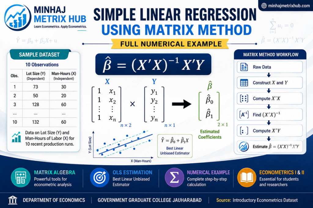
Simple Linear Regression Using Matrix: Full Numerical Example

Introduction: Why Use Matrix Algebra for Regression?

When we estimate a Simple Linear Regression Model (SLRM) using matrix algebra, we get a compact and generalizable method that extends easily to multiple regression. In this post, we solve a complete numerical example step by step — from setting up the data matrices to finding the OLS coefficients, predicted values, residuals, variance, standard errors, and $R^2$ .

Consider data on lot size ( $Y$ ) and man-hours of labor ( $X$ ) for 10 recent production runs. We want to estimate the OLS regression line $Y = \beta_0 + \beta_1 X + u$ using matrix notation.

Step 1: The Data

Run	Y (Lot Size)	X (Man-Hours)
1	73	30
2	50	20
3	128	60
4	170	80
5	87	40
6	108	50
7	135	60
8	69	30
9	148	70
10	132	60

Here $n = 10$ observations. In matrix form, the model is written as $Y = X\beta + u$ , where $Y$ is an $(n \times 1)$ vector, $X$ is an $(n \times 2)$ matrix (a column of 1’s for the intercept plus the values of the explanatory variable), $\beta$ is a $(2 \times 1)$ vector of parameters, and $u$ is the $(n \times 1)$ error vector.

Step 2: Setting Up the Y Vector and X Matrix

The $Y$ vector is:

$Y = \begin{bmatrix} 73 \\ 50 \\ 128 \\ 170 \\ 87 \\ 108 \\ 135 \\ 69 \\ 148 \\ 132 \end{bmatrix}$

The $X$ matrix (with a column of 1’s for the intercept term $\beta_0$ ) is:

$X = \begin{bmatrix} 1 & 30 \\ 1 & 20 \\ 1 & 60 \\ 1 & 80 \\ 1 & 40 \\ 1 & 50 \\ 1 & 60 \\ 1 & 30 \\ 1 & 70 \\ 1 & 60 \end{bmatrix}$

Step 3: Computing $X'X$

The transpose $X'$ is a $(2 \times 10)$ matrix:

$X' = \begin{bmatrix} 1 & 1 & 1 & 1 & 1 & 1 & 1 & 1 & 1 & 1 \\ 30 & 20 & 60 & 80 & 40 & 50 & 60 & 30 & 70 & 60 \end{bmatrix}$

Multiplying $X'X$ gives a $(2 \times 2)$ matrix made up of $n$ , $\sum X_i$ , and $\sum X_i^2$ :

$X'X = \begin{bmatrix} n & \sum X_i \\ \sum X_i & \sum X_i^2 \end{bmatrix}$

From the data: $\sum X_i = 500$ and $\sum X_i^2 = 28400$ . So:

$X'X = \begin{bmatrix} 10 & 500 \\ 500 & 28400 \end{bmatrix}$

Step 4: Computing $X'Y$

Multiplying $X'Y$ gives a $(2 \times 1)$ vector made up of $\sum Y_i$ and $\sum X_iY_i$ :

$X'Y = \begin{bmatrix} \sum Y_i \\ \sum X_iY_i \end{bmatrix}$

From the data: $\sum Y_i = 1100$ and $\sum X_iY_i = 61800$ . So:

$X'Y = \begin{bmatrix} 1100 \\ 61800 \end{bmatrix}$

Step 5: Finding the Inverse $(X'X)^{-1}$

For a $2 \times 2$ matrix $A = \begin{bmatrix} a & b \\ c & d \end{bmatrix}$ , the inverse is $A^{-1} = \frac{1}{|A|}\begin{bmatrix} d & -b \\ -c & a \end{bmatrix}$ , where $|A| = ad - bc$ .

First, the determinant of $X'X$ :

$|X'X| = (10)(28400) - (500)(500) = 284000 - 250000 = 34000$

Now the inverse:

$(X'X)^{-1} = \frac{1}{34000}\begin{bmatrix} 28400 & -500 \\ -500 & 10 \end{bmatrix}$

$(X'X)^{-1} = \begin{bmatrix} 0.835294 & -0.014706 \\ -0.014706 & 0.000294 \end{bmatrix}$

Step 6: Solving for the Coefficient Vector $\hat{\beta}$

The OLS coefficient vector is found from $\hat{\beta} = (X'X)^{-1}X'Y$ :

$\hat{\beta} = \begin{bmatrix} 0.835294 & -0.014706 \\ -0.014706 & 0.000294 \end{bmatrix}\begin{bmatrix} 1100 \\ 61800 \end{bmatrix}$

Solving element by element, using the exact fractions ( $\frac{1}{34000}$ ) to avoid rounding error:

$\hat{\beta}=(X'X)^{-1}X'Y=\frac{1}{34000}\begin{bmatrix}28400 & -500\\-500 & 10\end{bmatrix}\begin{bmatrix}1100\\61800\end{bmatrix}$

$\hat{\beta}_0 = \frac{(28400)(1100) + (-500)(61800)}{34000} = \frac{31{,}240{,}000 - 30{,}900{,}000}{34000} = \frac{340{,}000}{34000} = 10$

$\hat{\beta}_1 = \frac{(-500)(1100) + (10)(61800)}{34000} = \frac{-550{,}000 + 618{,}000}{34000} = \frac{68{,}000}{34000} = 2$

So the coefficient vector is:

$\hat{\beta} = \begin{bmatrix} \hat{\beta}_0 \\ \hat{\beta}_1 \end{bmatrix} = \begin{bmatrix} 10 \\ 2 \end{bmatrix}$

Step 7: The Estimated Regression Equation

Using the coefficients found above, the fitted regression line is:

$\hat{Y} = 10 + 2X$

This means for every additional man-hour of labor, lot size increases on average by 2 units, and the estimated lot size is 10 units when man-hours are zero (the intercept).

Step 8: Finding the Predicted Values $\hat{Y} = X\hat{\beta}$

The predicted values are obtained by multiplying the $X$ matrix by the coefficient vector $\hat{\beta}$ . Each row of $X$ is multiplied (as a dot product) with the column vector $\hat{\beta} = \begin{bmatrix} 10 \\ 2 \end{bmatrix}$ :

$\hat{Y} = X\hat{\beta} = \begin{bmatrix} 1 & 30 \\ 1 & 20 \\ 1 & 60 \\ 1 & 80 \\ 1 & 40 \\ 1 & 50 \\ 1 & 60 \\ 1 & 30 \\ 1 & 70 \\ 1 & 60 \end{bmatrix}\begin{bmatrix} 10 \\ 2 \end{bmatrix}$

Each element of $\hat{Y}$ is computed as $\hat{Y}_i = (1)(10) + (X_i)(2)$ , i.e., row $i$ of $X$ dotted with $\hat{\beta}$ :

$\hat{Y}_1 = 1(10) + 30(2) = 10 + 60 = 70$
$\hat{Y}_2 = 1(10) + 20(2) = 10 + 40 = 50$
$\hat{Y}_3 = 1(10) + 60(2) = 10 + 120 = 130$
$\hat{Y}_4 = 1(10) + 80(2) = 10 + 160 = 170$
$\hat{Y}_5 = 1(10) + 40(2) = 10 + 80 = 90$
$\hat{Y}_6 = 1(10) + 50(2) = 10 + 100 = 110$
$\hat{Y}_7 = 1(10) + 60(2) = 10 + 120 = 130$
$\hat{Y}_8 = 1(10) + 30(2) = 10 + 60 = 70$
$\hat{Y}_9 = 1(10) + 70(2) = 10 + 140 = 150$
$\hat{Y}_{10} = 1(10) + 60(2) = 10 + 120 = 130$

So the predicted values (fitted $Y$ ) matrix is:

$\hat{Y} = X\hat{\beta} = \begin{bmatrix} 70 \\ 50 \\ 130 \\ 170 \\ 90 \\ 110 \\ 130 \\ 70 \\ 150 \\ 130 \end{bmatrix}$

Step 9: Finding the Residual Matrix $e = Y - X\hat{\beta}$

The residual vector is found using the matrix equation $e = Y - X\hat{\beta} = Y - \hat{Y}$ , subtracting the predicted values matrix $\hat{Y}$ (Step 8) from the actual $Y$ matrix (Step 2), element by element:

$e = Y - X\hat{\beta} = \begin{bmatrix} 73 \\ 50 \\ 128 \\ 170 \\ 87 \\ 108 \\ 135 \\ 69 \\ 148 \\ 132 \end{bmatrix} - \begin{bmatrix} 70 \\ 50 \\ 130 \\ 170 \\ 90 \\ 110 \\ 130 \\ 70 \\ 150 \\ 130 \end{bmatrix} = \begin{bmatrix} 73-70 \\ 50-50 \\ 128-130 \\ 170-170 \\ 87-90 \\ 108-110 \\ 135-130 \\ 69-70 \\ 148-150 \\ 132-130 \end{bmatrix} = \begin{bmatrix} 3 \\ 0 \\ -2 \\ 0 \\ -3 \\ -2 \\ 5 \\ -1 \\ -2 \\ 2 \end{bmatrix}$

So the residual matrix is:

$e = \begin{bmatrix} 3 \\ 0 \\ -2 \\ 0 \\ -3 \\ -2 \\ 5 \\ -1 \\ -2 \\ 2 \end{bmatrix}$

For reference, the individual squared residuals used later in $e'e$ are:

Run	$Y$	$\hat{Y}$	$e = Y - \hat{Y}$	$e^2$
1	73	70	3	9
2	50	50	0	0
3	128	130	-2	4
4	170	170	0	0
5	87	90	-3	9
6	108	110	-2	4
7	135	130	5	25
8	69	70	-1	1
9	148	150	-2	4
10	132	130	2	4

Notice that $\sum e_i = 3+0-2+0-3-2+5-1-2+2 = 0$ , which confirms one of the key OLS properties — the sum of residuals is always zero. In matrix terms, this is because $\mathbf{1}'e = 0$ , i.e., the residual vector is orthogonal to the column of 1’s in $X$ .

Step 10: Residual Sum of Squares (RSS) — Two Matrix Approaches

Approach 1: Direct method, $e'e$

The residual sum of squares is found by pre-multiplying the residual vector by its transpose, $e'e$ :

$e'e = \sum e_i^2 = 9+0+4+0+9+4+25+1+4+4 = 60$

Approach 2: Matrix shortcut formula, $RSS = Y'Y - \hat{\beta}'X'Y$

This is the standard matrix formula used in econometrics, since $\hat{\beta}'X'Y = \hat{Y}'Y$ . First find $Y'Y$ (the sum of squared $Y$ values):

$Y'Y = \sum Y_i^2 = 73^2+50^2+128^2+170^2+87^2+108^2+135^2+69^2+148^2+132^2 = 134{,}660$

Next, find $\hat{\beta}'X'Y$ using the $\hat{\beta}$ vector and the $X'Y$ vector found in Step 4:

$\hat{\beta}'X'Y = \begin{bmatrix} 10 & 2 \end{bmatrix}\begin{bmatrix} 1100 \\ 61800 \end{bmatrix} = (10)(1100) + (2)(61800) = 11{,}000 + 123{,}600 = 134{,}600$

Therefore:

$RSS = Y'Y - \hat{\beta}'X'Y = 134{,}660 - 134{,}600 = 60$

Both approaches agree exactly: $RSS = 60$ .

Step 11: Total Sum of Squares (TSS) Using Matrices

The matrix formula for TSS is:

$TSS = Y'Y - \frac{(\mathbf{1}'Y)^2}{n} = Y'Y - n\bar{Y}^2$

where $\mathbf{1}'Y = \sum Y_i = 1100$ is the column of 1’s transposed and multiplied by $Y$ . First compute the correction term:

$\frac{(\mathbf{1}'Y)^2}{n} = \frac{(1100)^2}{10} = \frac{1{,}210{,}000}{10} = 121{,}000$

Now subtract from $Y'Y = 134{,}660$ (found in Step 10):

$TSS = 134{,}660 - 121{,}000 = 13{,}660$

This matches the direct computation $TSS = \sum(Y_i - \bar{Y})^2 = 13{,}660$ , confirming the result.

Step 12: Finding $R^2$ Using Matrices

Once RSS and TSS are both known from matrix operations (Steps 10 and 11), $R^2$ can be obtained entirely from matrix quantities—no need to touch the raw data again:

$R^2 = 1 - \frac{RSS}{TSS} = 1 - \frac{e'e}{Y'Y - n\bar{Y}^2}$

Substituting the matrix results already found:

$R^2 = 1 - \frac{60}{13{,}660} = 1 - 0.00439 = 0.9956$

Equivalently, $R^2$ can be written using the Explained Sum of Squares in matrix form, $ESS = \hat{\beta}'X'Y - n\bar{Y}^2$ :

$ESS = \hat{\beta}'X'Y - n\bar{Y}^2 = 134{,}600 - 121{,}000 = 13{,}600$

$R^2 = \frac{ESS}{TSS} = \frac{\hat{\beta}'X'Y - n\bar{Y}^2}{Y'Y - n\bar{Y}^2} = \frac{13{,}600}{13{,}660} = 0.9956$

Both matrix routes confirm $R^2 = 0.9956$ , meaning approximately 99.56% of the variation in lot size ( $Y$ ) is explained by man-hours of labor ( $X$ ).

Step 13: Variance and Standard Error of the Regression

The estimated variance of the error term (also called the Mean Square Error) is:

$\hat{\sigma}^2 = \frac{e'e}{n-k} = \frac{60}{10-2} = \frac{60}{8} = 7.5$

where $n - k = 8$ is the degrees of freedom ( $n=10$ observations, $k=2$ parameters estimated). The standard error of the regression (standard error of the estimate) is:

$\hat{\sigma} = \sqrt{7.5} = 2.7386$

Variance-Covariance Matrix of $\hat{\beta}$

The variance-covariance matrix of the coefficient estimates is given by $Var(\hat{\beta}) = \hat{\sigma}^2 (X'X)^{-1}$ :

$Var(\hat{\beta}) = 7.5 \begin{bmatrix} 0.835294 & -0.014706 \\ -0.014706 & 0.000294 \end{bmatrix} = \begin{bmatrix} 6.26471 & -0.11029 \\ -0.11029 & 0.00221 \end{bmatrix}$

The standard errors of the coefficients are the square roots of the diagonal elements:

$se(\hat{\beta}_0) = \sqrt{6.26471} = 2.5029$

$se(\hat{\beta}_1) = \sqrt{0.00221} = 0.0470$

Step 14: Testing Significance — The t-Values

To test whether each coefficient is statistically significant, we compute the t-statistic for each parameter using:

$t_{\hat{\beta}_j} = \frac{\hat{\beta}_j}{se(\hat{\beta}_j)}$

Using $\hat{\beta}_0 = 10$ , $se(\hat{\beta}_0) = 2.5029$ (from Step 13):

$t_{\hat{\beta}_0} = \frac{10}{2.5029} = 3.9953$

Using $\hat{\beta}_1 = 2$ , $se(\hat{\beta}_1) = 0.0470$ (from Step 13):

$t_{\hat{\beta}_1} = \frac{2}{0.0470} = 42.5833$

With $n - k = 8$ degrees of freedom, the critical value from the t-table at the 5% level of significance (two-tailed test) is $t_{0.025,8} = 2.306$ .

Interpretation of Significance

Since $|t_{\hat{\beta}_0}| = 3.9953 > 2.306$ , the intercept $\hat{\beta}_0$ is statistically significant at the 5% level — it is significantly different from zero.

Since $|t_{\hat{\beta}_1}| = 42.5833 > 2.306$ , the slope $\hat{\beta}_1$ is highly statistically significant, well beyond even the 1% level ( $t_{0.005,8} = 3.355$ ). This provides very strong evidence that man-hours of labor has a real and precise positive effect on lot size, and the relationship is extremely unlikely to be due to chance.

In short, both coefficients pass the significance test, but the slope coefficient’s exceptionally high t-value (42.58) reflects the near-perfect linear fit already suggested by $R^2 = 0.9956$ .

Summary of Results

Statistic	Value
Intercept ( $\hat{\beta}_0$ )	10
Slope ( $\hat{\beta}_1$ )	2
Regression Equation	$\hat{Y} = 10 + 2X$
Residual Sum of Squares (RSS)	60
Total Sum of Squares (TSS)	13,660
Explained Sum of Squares (ESS)	13,600
Variance ( $\hat{\sigma}^2$ )	7.5
Standard Error of Regression ( $\hat{\sigma}$ )	2.7386
Standard Error of $\hat{\beta}_0$	2.5029
Standard Error of $\hat{\beta}_1$	0.0470
Coefficient of Determination ( $R^2$ )	0.9956
t-value of $\hat{\beta}_0$	3.9953
t-value of $\hat{\beta}_1$	42.5833
Critical t-value ( $\alpha=0.05$ , df=8)	2.306
Significance	Both coefficients significant at 5%

Conclusion

Using matrix algebra, we estimated the simple linear regression of lot size on man-hours of labor and found $\hat{Y} = 10 + 2X$ . The very high $R^2$ of 0.9956 and the small standard errors of both coefficients suggest that man-hours of labor is a strong and precise predictor of lot size in this production process. This same matrix approach — $\hat{\beta} = (X'X)^{-1}X'Y$ — extends directly to multiple regression with any number of explanatory variables, which is why it forms the foundation of econometric estimation.

Frequently Asked Questions

Q1: Why do we add a column of 1’s in the X matrix?
The column of 1’s allows the matrix multiplication to generate the intercept term $\beta_0$ automatically as part of the coefficient vector, rather than estimating it separately.

Q2: Why is $\sum e_i = 0$ in every OLS regression?
This is a mathematical property of the OLS normal equations: since the first normal equation sets $\sum e_i = 0$ , minimizing the sum of squared residuals always forces residuals to sum to zero when an intercept is included in the model.

Q3: What does a high $R^2$ value of 0.9956 mean?
It means that 99.56% of the variation in the dependent variable (lot size) is explained by the independent variable (man-hours of labor), leaving only 0.44% unexplained by the model.

Q4: Why divide by $n-k$ instead of $n$ when calculating variance?
Dividing by $n-k$ (degrees of freedom) instead of $n$ corrects for the bias introduced by estimating $k$ parameters from the sample, giving an unbiased estimator of the error variance $\sigma^2$ .

Q5: How is the matrix method different from the direct-formula method of SLRM?
Both methods give identical results for simple regression. The matrix method, however, is more general — it applies directly to multiple regression with several explanatory variables using the same formula $\hat{\beta} = (X'X)^{-1}X'Y$ , without needing separate formulas for each parameter.

Q6: Why does the matrix shortcut $RSS = Y'Y - \hat{\beta}'X'Y$ give the same answer as $e'e$ ?
Because $\hat{\beta}'X'Y$ is algebraically equal to $\hat{Y}'Y$ , the fitted values dotted with actual $Y$ . Since $e'e = (Y-\hat{Y})'(Y-\hat{Y}) = Y'Y - 2\hat{Y}'Y + \hat{Y}'\hat{Y}$ , and OLS properties make $\hat{Y}'\hat{Y} = \hat{Y}'Y$ , the expression simplifies exactly to $Y'Y - \hat{\beta}'X'Y$ .

Q7: What does a very high t-value like 42.58 for the slope mean?
A large t-value means the estimated coefficient is many standard errors away from zero, so we can be extremely confident the true slope is not zero. It signals a strong, precisely estimated relationship between man-hours of labor and lot size, consistent with the very high $R^2$ .

Suggestions for further readings:

The Matrix Algebra of Linear Regression | Towards Data Science

Share this article

Leave a Reply Cancel reply

Dummy Variable Regression Model Explained with Solved Examples

Dummy Variable Regression Model: A Complete Guide with Solved Examples In basic regression analysis, we

August 5, 2026 No Comments

Derivation of OLS Estimator in Matrix Form

Econometrics

Derivation of OLS Estimator in Matrix Form

Matrix Approach to Linear Regression Model The K-Variable Linear Regression Model Consider the following K-variable

August 4, 2026 No Comments

Autocorrelation in Econometrics: Causes, Consequences, Detection, and Remedies

Autocorrelation in Econometrics Causes, Consequences, Detection, and Remedies Much of applied macroeconomic research, from modelling

July 27, 2026 No Comments

Econometrics

Heteroscedasticity in Econometrics: Meaning, Causes, Tests, and Remedies Explained

Heteroscedasticity in Econometrics: Meaning, Causes, Tests, and Remedies Explained One of the core assumptions of

July 19, 2026 No Comments

Econometrics

Methodology of Econometrics: 8 Steps Explained with Example

Methodology of Econometrics: 8 Steps Explained with an Example Every empirical study in economics, whether

July 17, 2026 No Comments

Muhammad Minhaj Akhtar

Muhammad Minhaj Akhtar is a Lecturer in Economics at Government Graduate College Jauharabad, Pakistan. He holds an M.Phil. in Economics from Quaid-i-Azam University, Islamabad, and an MSc in Economics from the University of Sargodha, where he earned a Silver Medal. His academic passion lies in Econometrics, with a strong focus on applying empirical methods to real-world economic issues. Through MinhajMetrixHub, he shares learning resources, research guidance, and practical econometric insights for students and researchers.

Simple Linear Regression Using Matrix: Full Numerical Example